On Position Letter Frequency

Interactive website: letter-frequency.com

My primary inspiration for this was reading a passage from Thinking Fast and Slow by Daniel Kahneman:

In one of our studies, we asked participants to answer a simple question about words in a typical English text:

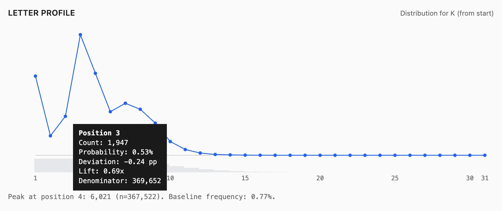
Consider the letter K. Is K more likely to appear as the first letter in a word OR as the third letter?

As any Scrabble player knows, it is much easier to come up with words that begin with a particular letter than to find words that have the same letter in the third position. This is true for every letter of the alphabet. We therefore expected respondents to exaggerate the frequency of letters appearing in the first position—even those letters (such as K, L, N, R, V) which in fact occur more frequently in the third position. Here again, the reliance on a heuristic produces a predictable bias in judgments.

This got me curious, i wanted to see numerically how letter distributions shift by position and study patterns like which tend to occur early vs late. I’m sure there are hundreds if not thousands of studies on this, but I still wanted to build it myself.

Data

I used a wordlist-style dataset from dwyl/english-words (words_alpha.txt), with observed maximum length 31, totalling 3,494,700 letter tokens across all positions.

A wordlist is not a typical English text. It weights rare words the same as common word. A corpus would be more faithful to actual reading experience, but the wordlist is a great starting point especially for exploring structure.

Counting

For each position $i$ (1..31) and each letter $\ell$ (a..z), I want:

• count(i, ℓ): number of words whose $i$-th letter is $\ell$
• total(i): number of words long enough to have an $i$-th letter
• probability(i, ℓ) = count(i, ℓ) / total(i)

This naturally forms a matrix: 31 positions x 26 letters

total is not constant. It decreases with position, because fewer words are long enough to reach deeper positions. If you don’t keep that denominator in view, later positions can produce visually dramatic (but statistically fragile) spikes.

Algorithm

The algorithm is a single pass over all words:

1. Allocate two arrays:

   • counts[i][ℓ] counts per position/letter
   • totals[i] how many words contribute to that position

2. For each word $w$:

   • for each index i in the word:
     • increment totals[i]
     • increment counts[i][letter]

$$O\left(\sum_{w \in \text{words}} |w|\right)$$

Memory is fixed, 31 x 26 integers plus a small totals array.

Implementation

Here’s the core counting function plus CSV emission

func countPositional(words []string) (counts [][]int, totals []int) {
	maxLen := 0
	for _, w := range words {
		if len(w) > maxLen { maxLen = len(w) }
	}
	counts = make([][]int, maxLen)
	totals = make([]int, maxLen)
	for i := range counts { counts[i] = make([]int, 26) }

	for _, w := range words {
		for i := 0; i < len(w); i++ {
			c := w[i]
			if c < 'a' || c > 'z' {
				continue
			}

			totals[i]++
			counts[i][c-'a']++
		}
	}

	return counts, totals
}

func writeCSV(w io.Writer, counts [][]int, totals []int) {
	fmt.Fprintln(w, "position,letter,count,total_at_position,probability")
	for i := 0; i < len(counts); i++ {
		total := totals[i]
		for l := 0; l < 26; l++ {
			c := counts[i][l]
			p := 0.0
			if total > 0 { p = float64(c) / float64(total) }
			fmt.Fprintf(w, "%d,%c,%d,%d,%.10f\n", i+1, byte('a'+l), c, total, p)
		}
	}
}

A note on denominators, i increment totals[i] only when the character is in a..z, so total_at_position(i) is words that contribute a valid letter at that position. This assumes the dataset is already clean which word_alpha.txt is. If you had hyphens and apostrophes, you’d need to decide whether to (a) drop those words, (b) treat punctuation as a character, or (c) count letter-only positions where you skip non-letters.

I also implemented the same counting from the end (last letter, second-to-last, …) to study suffix-driven structure. I’m not including those results here, but the idea is straightforward: when scanning a word, map each character’s index to a distance from end index instead of a from start index.

The dataset has a median word length of 9 and p90 is 13. That means by the time you’re analysing position 15+, you’re already into long word territory and a few weird words can distort the picture.

For any strong claims or most extreme summaries, I set a simple guard to only treat a position as reliable if total_at_position(i) >= 1000

In this dataset, position 1-19 clear that threshold; position 20 drops to 660.

Findings

In this wordlist:

• K at position 1 is at 1.07%
• K at position 3 is at 0.53%

So we can infer for K specifically, it’s really is more common to be at the first position than third. Also K peaks at the fourth position.

But Kahneman’s broader point (some letters occurs more at position 3 than position 1) though shows up clearly. For example:

• N: 3.64% (pos1) vs 8.84% (pos3)
• R: much higher at pos3 than pos1
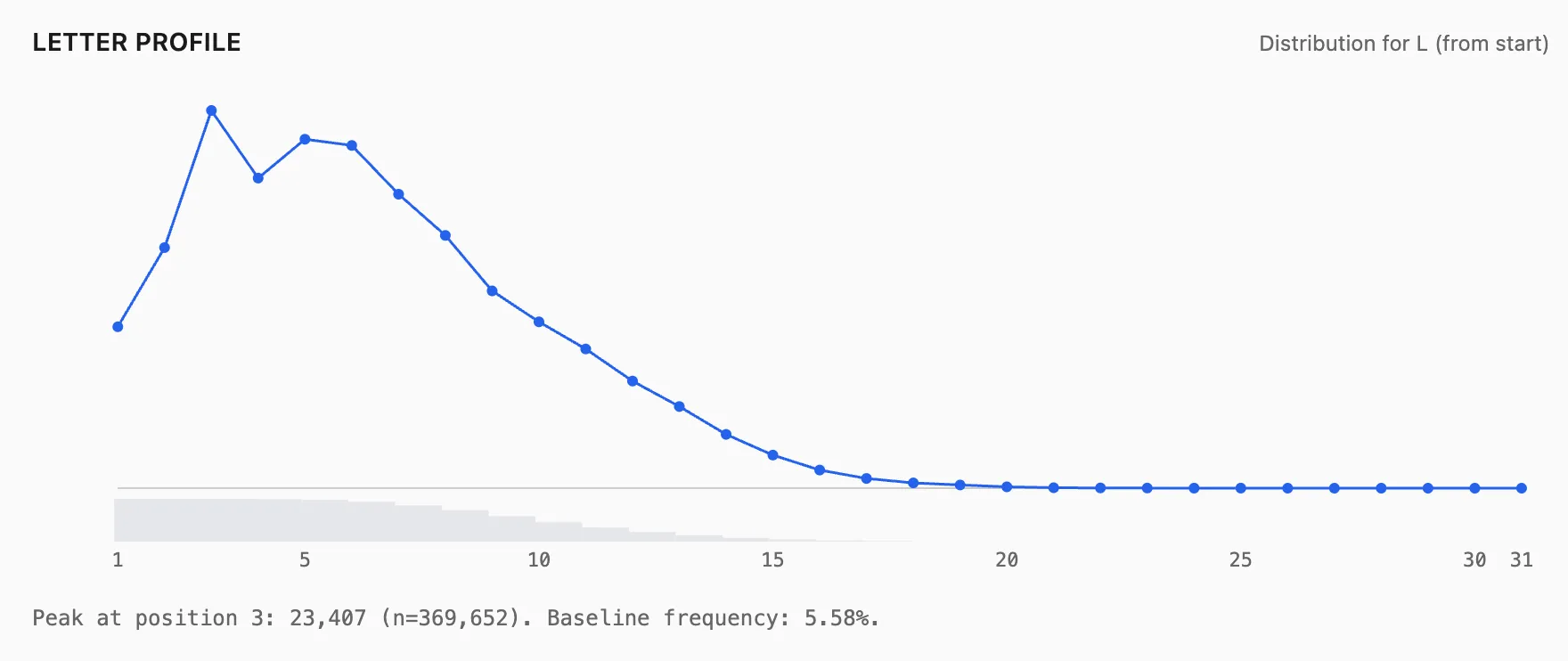
• L: much higher at pos3 than pos1

In other words, intuition about first letters is strong but the correct answer depends on the letter.

Talking about Position 1, two examples that jumped out immediately:

• P is extremely common as a first letter: 9.419% at position 1. Its overall baseline frequency is only 3.252%.
• E suprisingly is somewhat underrepresented as a first letter: 3.836% at position 1. Its baseline is 10.772%.

So if all you know are overall letter frequencies (ETAOIN…), you might guess the first letter distribution is a mild variation of the baseline. It isn’t. The start of words has its own structure, some letters are unusually good starters, and some are surprisingly rare at position 1 relative to how common they are overall.

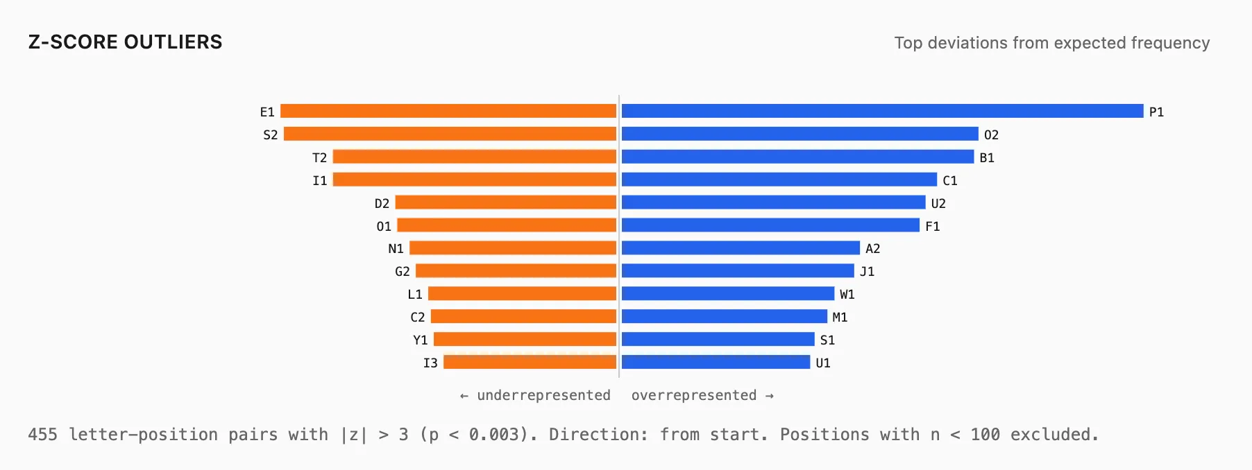
At position 2, there’s a notable spike:

• O at position 2 is very high (13.34% vs 7.20% baseline)

⠀…and some letters drop sharply from position 1:

• S at position 2 is very low (1.45% vs 7.16% baseline)

This lines up with common English orthographic pattern, we have many starts like co-, en-, bi- and comparatively fewer words where s is the second character.

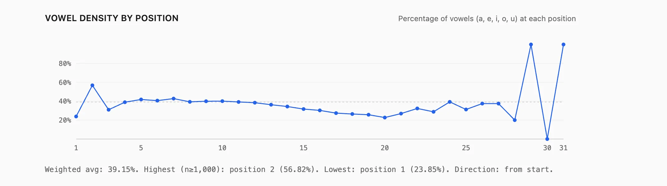
If you aggregate vowels (a, e, i, o, u), the same need a vowel early pattern shows up strongly. Among positions with enough data (n ≥ 1000), vowel density is highest at position 2 (around 56.82%) and lowest at position 1 (around 23.85%).

English words often start with a consonant, and then quickly need a vowel to become pronounceable.

As you go deeper into a word, the distribution becomes more constrained. One way to quantify that is Shannon entropy: high entropy means lots of plausible letters, lower entropy means the position is predictable.

In this dataset, entropy trends downward as position increases:

• early positions have many plausible letters
• later positions narrow because spelling conventions and morphology constrain what’s plausible

How you average entropy matters though

• An unweighted average treats position 31 (tiny sample) the same as position 1 (370k words).
• A weighted average (what I switched to) reflects what you’d see if you sampled a random positioned letter token.

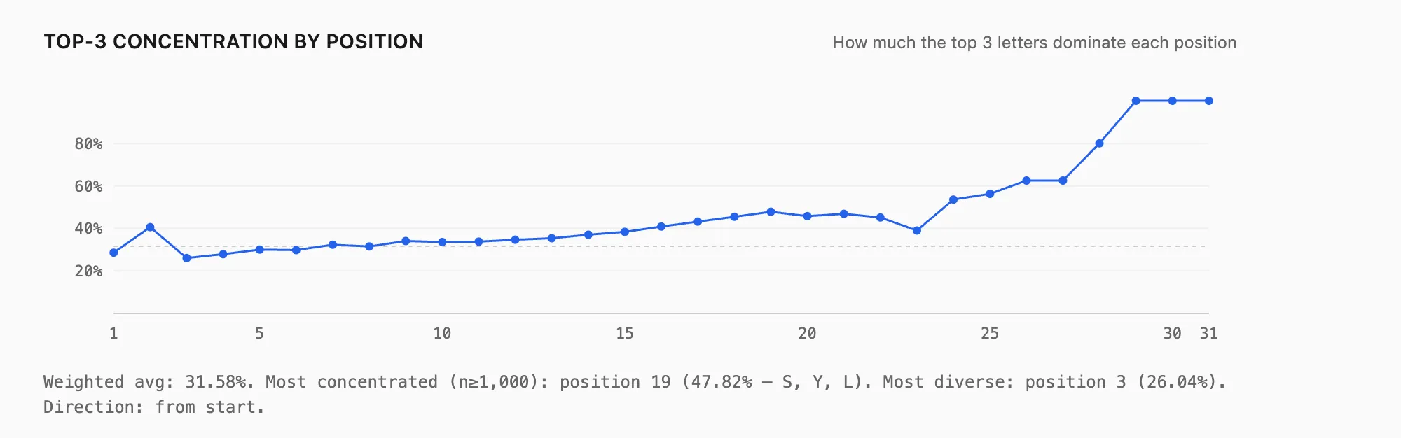
A related signal is concentration i.e how dominated is this position by just a few letters? Looking at the combined probability of the top 3 letters at each position, concentration rises as you move later into words, even before the extreme tail. That’s consistent with suffix patterns taking over.

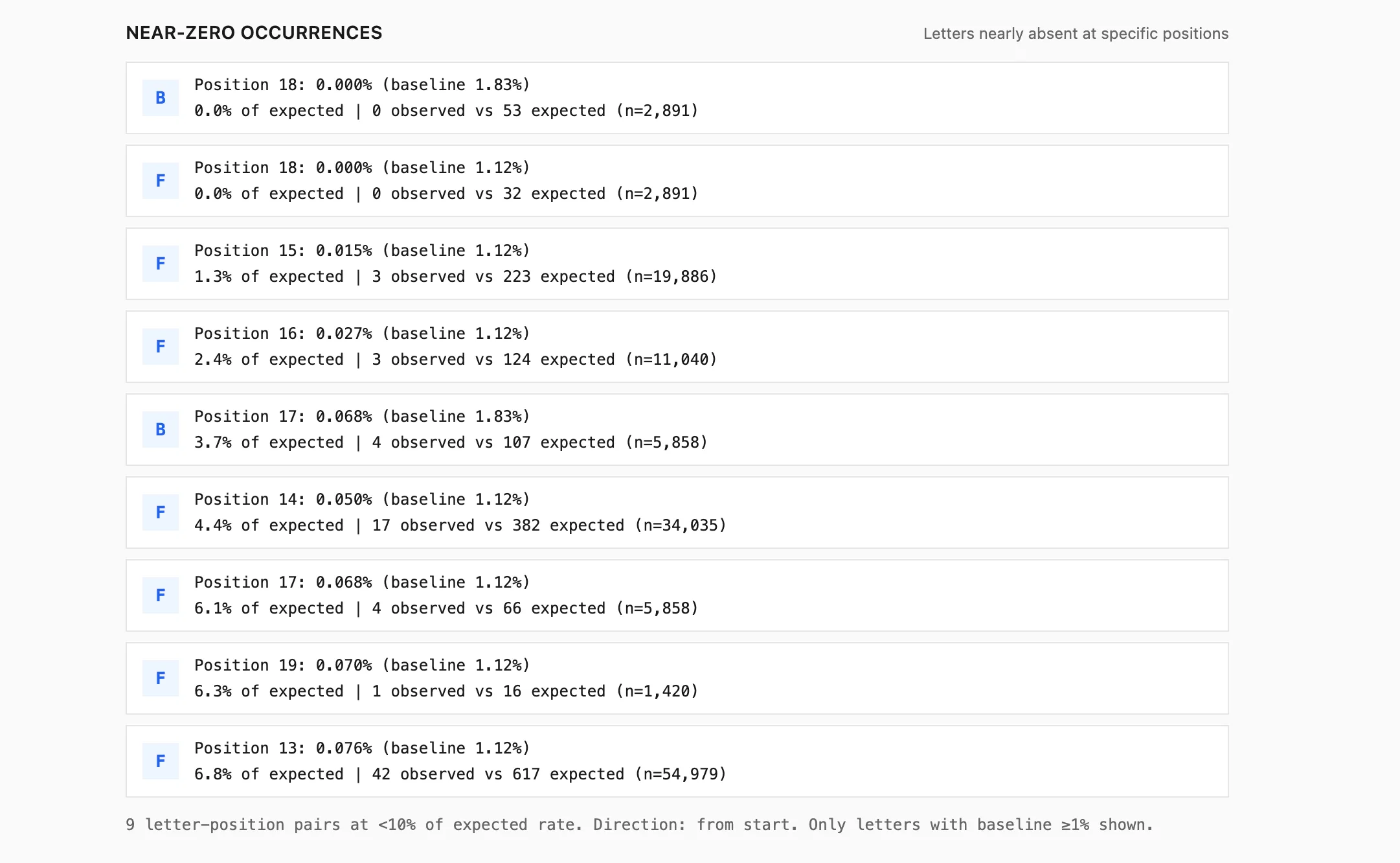
Finally, you can look for near-impossible combinations i.e letter position pairs that occur at less than 10% of their expected rate (relative to baseline), restricted to common letters and reliable positions. These often point to orthographic/morphological constraints rather than just noise.

Closing

This article only scratches the surface. If you want to dig around interactively; switch letters, positions, metrics, and compare from start vs from end I’ve put the full explorer here letter-frequency.com and code here

If you replicate this with a frequency weighted corpus (books, news, subtitles), I’d expect the broad structural patterns to remain (vowel pressure early, suffix constraints late), but the magnitudes and the most extreme outliers will change, because wordlists overweight rare and archaic forms.

If you do try it with a different corpus, the easiest sanity check is the denominator is always keep total_at_position(i) in view, and be skeptical of any dramatic pattern in the tail where the sample size collapses.